How to protect data in Google Sheets

When you’ve got important data and want to share it with colleagues, protecting your spreadsheets is important. Here’s how to protect your data.

Mar 3, 2024 - 02:30

0 9

When you have vast amounts of data, making a change by mistake can throw off your calculations or projections, or might misinform. Protecting your data from accidental changes will ensure that your information is correct and free of error.

Protecting your data is also helpful when you’re sharing a spreadsheet with colleagues and friends, who can help you review your data without having them make any changes.

How to protect your data

In Google Sheets, you can protect your data in two ways: by spreadsheet or by range. To protect your spreadsheet in Google Sheets, go to “Data” in the menu bar, and then click on “Protect sheet and ranges.”

The selection is defaulted to “Range,” and the field below it lists the spreadsheet and the range of data. You can change the data range directly, or you can click on the four-grid icon to the right to allow you to pick the range of data by highlighting specific fields in the spreadsheet.

To protect the entire spreadsheet, click on “Sheet” in the “Protect sheets & ranges” selection, and that will list the name of the spreadsheet, which will list the same name that appears as a tab on the lower left of the screen.

After picking either “Range” or “Sheet,” you’ll have to click on “Set permissions” to establish what kind of restrictions apply. After clicking on “Set permissions,” a window appears to initiate the authorization.

The default selection is “Restrict who can edit this range” followed below by “Only you.” You can grant permission to other persons by selecting “Custom” and putting in their email addresses. That will allow those persons to edit by sharing the link.

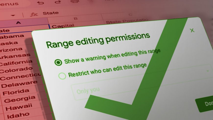
The downside to selecting yourself as editor of your protected worksheet is that you might make accidental changes without realizing what you’re doing. The alternative is to select “Show a warning when editing this range” in the “Range editing permissions” under “Set permissions.”

This functionality creates a warning in a new pop-up window with a tag at the top that says “Heads up!” You’re overriding or entering new data onto a particular field in the spreadsheet, and it either lets you cancel or proceed by clicking “OK.”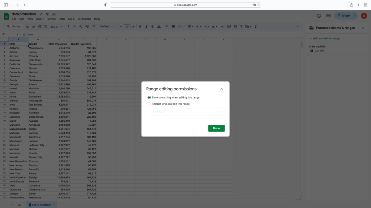

You can protect a range of cells in a spreadsheet or the spreadsheet itself. Protecting data can prevent correcting errors down the road.
Google Sheets

Example of data protection

Using the same spreadsheet used in the data sorting tutorial on states, their capitals, and populations, we will protect the data by range and spreadsheet. Following the same steps above, we will go to “Data” in the menu bar and select “Protect sheet and ranges.”

The spreadsheet version of the following tutorial can be downloaded here. Make a copy of the worksheet by selecting "Make a copy" from the drop-down in the File menu.

To the right of the spreadsheet, a sidebar titled “Protected sheets & ranges” pops up. Click on “Add a sheet or range” below that, and from there, the default setting is “Range” with the name of the spreadsheet in single quotes followed by an exclamation mark and a cell. For the cell range selection, type in “A1:D51” so that the field reads “ 'state capitals'!A1:D51.” This will protect the data by state, capital, state population, and capital population, including the headers at Row 1.

Click on “Set permissions” and another window titled “Range editing permissions” pops up. Pick “Show a warning when editing this range,” and click “Done.” The range from A1 to D51 is now protected, and any attempt to change a text will trigger a warning to appear.

To protect the entire spreadsheet, click on “Sheet” under “Protected sheets & ranges,” and the name of the spreadsheet, “state capitals,” appears in the field. Click “Set permissions.” In the window pop-up, pick “Show a warning when editing this range,” and click “Done.” The entire spreadsheet titled “state capitals” is now protected. Any entry in any cell in the spreadsheet will automatically trigger an alert.

Watch: How to protect data in Google Sheets

Again, the spreadsheet version of the following tutorial can be downloaded here. Make a copy of the worksheet by selecting "Make a copy" from the drop-down in the File menu.

This is just one of many articles about easy-to-use tools in Google Sheets. See more below from TheStreet.

Let us know what you'd like to see next. Email us here: [email protected]

Original Post